Unfucking audio with "AI"

Thursday February 20 2025, 1434 words — Using machine learning to unfuck broken audio recordings.
Filed under: Software, Machine Learning, Audio

Ok, I fucking hate “AI” and the corporate horse it rode in on. Machine learning though? I guess that’s kinda useful?!

I’ve been helping out my friends at KKTO with their project Minute/Year for almost a decade now and a while ago we had run into a peculiar problem. I spent the last few days finally cleaning up the mess it caused and I thought I’d write up what I’ve done cause I’m pretty proud of the result.

In 2023 an audio interface had failed and corrupted a whole bunch of our daily recordings in a subtle yet annoying way. It took us a few days to realize what had happened at which point we power cycled the audio interface and everything went back to normal but it left us with a bunch of corrupted recordings that needed to be fixed.

What had happened

The installation records a single minute of audio every day and creates a spectrogram of said recording as part of the process. Looking at the spectrogram it wasn’t hard to see that something was… off.

These spectrograms show the change of frequencies in the recording over time, low frequencies at the bottom, high frequencies at the top. The scale is linear, with the top frequency maxing out at 24kHz. Not only was there a lot more high frequency content than usual the whole thing also looked suspiciously… mirrored.

This got my aliasing senses tingling.

And would you look at that. For some reason every second sample in recording was just a copy of the previous one. Effectively cutting our sample rate in half and causing a ton of aliasing!

To be honest, I have no idea what happened here. For some reason the audio interface just started doubling up samples at some point. And since we couldn’t repeat the recordings it was my task to fix them up as best as possible.

Identifying affected recordings

Since I wanted to make completely sure I wouldn’t miss any corrupted recordings I wrote a quick python script to iterate over all of the 2023 recordings and identify the corrupted ones.

recordings = glob.glob("[0-9][0-9][0-9].wav", root_dir="recordings")
recordings.sort()

bad_recordings = []
good_recordings = []
for file in recordings:
	data, _ = sf.read(f"recordings/{file}")
	data = data.T

	# Combine both channels into a single mono channel
	left = data[0]
	right = data[1]
	mono = data[0] + data[1]

	# Subtract every pair of samples from each other
	diff_even = np.abs(np.average(mono[50000:-50000:2] - mono[50001:-50000:2]))
	diff_odd = np.abs(np.average(mono[50001:-50001:2] - mono[50002:-50000:2]))

	# Find the ones where either difference is always zero
	if diff_even == 0 or diff_odd == 0:
		print(f"{file}: {diff_even} {diff_odd}")
		bad_recordings += [file]
	else:
		good_recordings += [file]

This piece of code finds all recordings using python’s built in glob module, sorts them, loads them using PySoundFile and does some quick analysis using numpy.

It mainly boils down to taking the difference between every sample and it’s successor. This needs to be done both for even and odd offsets since we can’t be entirely sure if the file begins with a repeated sample or not. I’m also cutting out the first and last 50k samples from each recording since the files had a fade in and out applied in post, so these sections wouldn’t be exactly as they came from the audio interface.

Using this approach I identified a total of 15 corrupted recordings.

Let’s fix them!

The naive approach

Ok, so, at this point the easiest solution would be to just throw out all the doubled up samples and resampling the recordings back to their original length. This can be easily done with another piece of python code with the help of scipy.signal.

for file in bad_recordings:
	print(f"Fixing: {file}")
	data, sample_rate = sf.read(f"recordings/{file}")
	data = data.T

	orig_len = len(data[0])

	# Discard every second sample
	left = data[0,0::2]
	right = data[1,0::2]

	# Resample to original length
	left_fixed = sig.resample(left, orig_len)
	right_fixed = sig.resample(right, orig_len)

	fixed_data = np.stack((left_fixed, right_fixed)).T
	sf.write(f"fixed/{file}", fixed_data, sample_rate, subtype="FLOAT")

This works but has one major flaw. It results in half the spectrum basically being completely blank without any sign of the noise that would usually be present in a recording like this. It also limits our frequency range to just 12kHz.

Now, a reasonable thing to say here might be “Well, this is the best we can do! All the original high frequency information was lost anyways!”.

And while that’s true we don’t really need the original high frequency content. We just need to make some up that’s plausible enough! And what’s really good at making up stuff that seems plausible enough?

“Fixing” it with machine learning

I’ve done some work with tensorflow before but I’ve always found it a huge pain to set up. Case in point this time it just flat out refused to work because my distribution (I use arch by the way) doesn’t ship the same old version of python that tensorflow needs.

So I decided to give pytorch a try instead. I figured it’d be similar enough and it could just be installed into a venv using pip.

Gathering training data

The first step would be to gather some training data of similarly messed up files to train a neural network on. Luckily I had around 350 uncorrupted recording from the same year which I could artificially introduce the same error into and use as training data.

I basically used the same code as I used above to find the corrupted files but this time I collected all the uncorrupted files and built a dataset from them.

fft_size = 2048

for file in good_recordings:
	data, _ = sf.read(f"recordings/{file}")
	data = data.T

	left = data[0]
	right = data[1]

	# Create corrupted version of recording by overwriting every second sample with it's neighbor
	corrupted_left = np.copy(left)
	corrupted_left[0::2] = left[1::2]
	corrupted_right = np.copy(right)
	corrupted_right[0::2] = right[1::2]

	# Create STFT spectrogram of original recording
	_, _, spec_l = sig.stft(left, nperseg=fft_size)
	_, _, spec_r = sig.stft(right, nperseg=fft_size)
	spec_l = lin_to_db(np.abs(spec_l.T))
	spec_r = lin_to_db(np.abs(spec_r.T))

	# Create STFT spectrogram of corrupted recording
	_, _, spec_l_corrupted = sig.stft(corrupted_left, nperseg=fft_size)
	_, _, spec_r_corrupted = sig.stft(corrupted_right, nperseg=fft_size)
	spec_l_corrupted = lin_to_db(np.abs(spec_l_corrupted.T))
	spec_r_corrupted = lin_to_db(np.abs(spec_r_corrupted.T))

	# Add pairs of corrupted and uncorrupted spectrogram time slices to data set
	dataset_add(np.stack((spec_l_corrupted, spec_l), axis=1))
	dataset_add(np.stack((spec_r_corrupted, spec_r), axis=1))

The function dataset_add() just dumps all the pairs of STFT time slices into a large HDF5 dataset for storage.

You’ll notice that I discard all phase information from the spectral data and just store the magnitudes on a logarithmic scale. I found that the learning goes a lot easier with the magnitudes on a log scale than a linear one. And I’ll get around to why I didn’t keep the phase information later.

Building a neural network

So, building neural networks is hard, I heard. A whole science in itself. So in consideration for my own time and energy I just did the dumbest thing possible.

class FlatNet(nn.Module):
	def __init__(self, fft_size):
		super().__init__()
		self.linear = nn.Linear(fft_size, fft_size)

	def forward(self, x):
		return self.linear(x)

Yep, it’s just a single fully connected layer. I call it “Shallow Learning”.

I tried a bunch of more complex networks first but training them on my ancient CPU took ages. This one worked way better than it had any right to and was done training in just around five hours.

Here is the abridged training code I used, copied pretty much straight from one of the pytorch examples:

model = FlatNet(fft_size)
model.train()

criterion = nn.MSELoss()
optimizer = optim.Adam(model.parameters(), lr=1e-5)

while not done:
	for data in dataset:
		corrupted = data[:,0,:]
		clean = data[:,1,:]
		optimizer.zero_grad()

		pred = model(corrupted)
		loss = criterion(pred, clean)
		loss.backward()
		optimizer.step()

As you can see I used a simple mean squared error loss metric and an adam optimizer with a learning rate of of 1×10^-5.

Let’s take a look at some graphs! Everybody loves graphs!

The frequency plots show the uncorrupted spectrogram in orange, the corrupted one in blue and the reconstruction by the neural network in green.

As you can see the approximation is pretty damn good. The spectrum in the high frequencies tends a little towards being too smooth but it doesn’t make a big difference in the final files. One of the most impressive things is visible in the last graph from still pretty early in the training process. Not only is it able to recreate the high frequency spectrum but it also correctly removes the aliased frequencies from the low end! I did not expect that to work!

Unfucking the recordings

At this point the only step that remains is to use the freshly trained network to unfuck the recordings!

for file in bad_files:
	data, sample_rate = sf.read(f"recordings/{file}")
	data = data.T

	orig_len = len(data[0])

	left = data[0]
	right = data[1]

	# Generate STFT spectrogram of corrupted file, storing the phases for later
	_, _, spec_l = sig.stft(left, fs=sample_rate, nperseg=fft_size)
	_, _, spec_r = sig.stft(right, fs=sample_rate, nperseg=fft_size)
	phases_l = np.angle(spec_l.T)
	phases_r = np.angle(spec_r.T)
	mags_l = lin_to_db(np.abs(spec_l.T))
	mags_r = lin_to_db(np.abs(spec_r.T))

	# Apply neural network to magnitudes
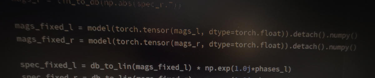
	mags_fixed_l = model(torch.tensor(mags_l, dtype=torch.float)).detach().numpy()
	mags_fixed_r = model(torch.tensor(mags_r, dtype=torch.float)).detach().numpy()

	# Combine new magnitudes with original phase information
	spec_fixed_l = db_to_lin(mags_fixed_l) * np.exp(1.0j*phases_l)
	spec_fixed_r = db_to_lin(mags_fixed_r) * np.exp(1.0j*phases_r)

	spec_fixed_l = spec_fixed_l.T
	spec_fixed_r = spec_fixed_r.T

	# Do a reverse STFT
	_, left_fixed = sig.istft(spec_fixed_l, fs=sample_rate)
	_, right_fixed = sig.istft(spec_fixed_r, fs=sample_rate)

	# Crop recordings to original length to get rid of padding
	left_fixed = left_fixed[:orig_len]
	right_fixed = right_fixed[:orig_len]

	# Put everything into a new wave file
	fixed_data = np.stack((left_fixed, right_fixed)).T
	sf.write(f"fixed/{file}", fixed_data, sample_rate, subtype="FLOAT")

As you can see we first generate an STFT spectrogram of the wave data just like we did for the training data, but this time I make sure to keep the phase information. Since the neural network doesn’t touch the phase information we’ll just reuse the original phases for the reconstruction. For the low frequency content that’s gonna be close enough and for the high frequency content it doesn’t really matter.

So, how well does it work? Really well! See for yourself!

Conclusion

So while it seems that right now most of the conversation about “AI” is dominated by grifters set on boiling the oceans I think there is some genuinely really useful and cool stuff you can do with machine learning, even on a tiny scale that runs on a computer from 2012.

I think it’s time to bring back bad machine learning. The trippy puppy slugs and terrifying synthesized voices from hell. I’m doing my part.